ตอนนี้เราพร้อมที่จะพิจารณาการออกแบบ nonrecursive filter อย่างเป็นระบบแล้ว วิธีการออกแบบนี้มีพื้นฐานมาจาก Figure 16.1 ซึ่งประกอบด้วยหกส่วน ที่มุมซ้ายบนคือภาพร่างของ ideal filter ที่คุณต้องการ มันสามารถเป็น low-pass, high-pass, band-pass, band-stop, notch filter หรือแม้กระทั่ง differentiator สำหรับสิ่งอื่นที่ไม่ใช่ differentiator filter โดยปกติคุณต้องการให้ความสูงเป็น 0 หรือ 1 ในช่วงต่างๆ ขณะที่สำหรับ differentiator คุณต้องการ iω เนื่องจากอนุพันธ์ของ eigenfunction คือ

ดังนั้น eigenvalue ที่ต้องการคือสัมประสิทธิ์ iω สำหรับ differentiator มักจะมี cutoff ที่ความถี่หนึ่งเพราะอย่างที่คุณเห็น การทำ differentiation จะขยายสัญญาณ คูณด้วย ω และจะมีค่ามากขึ้นที่ความถี่สูง ซึ่งมักจะเป็นที่ที่ noise อยู่ Figure 16.2 ดูเพิ่มเติมที่ Figure 15.2 .
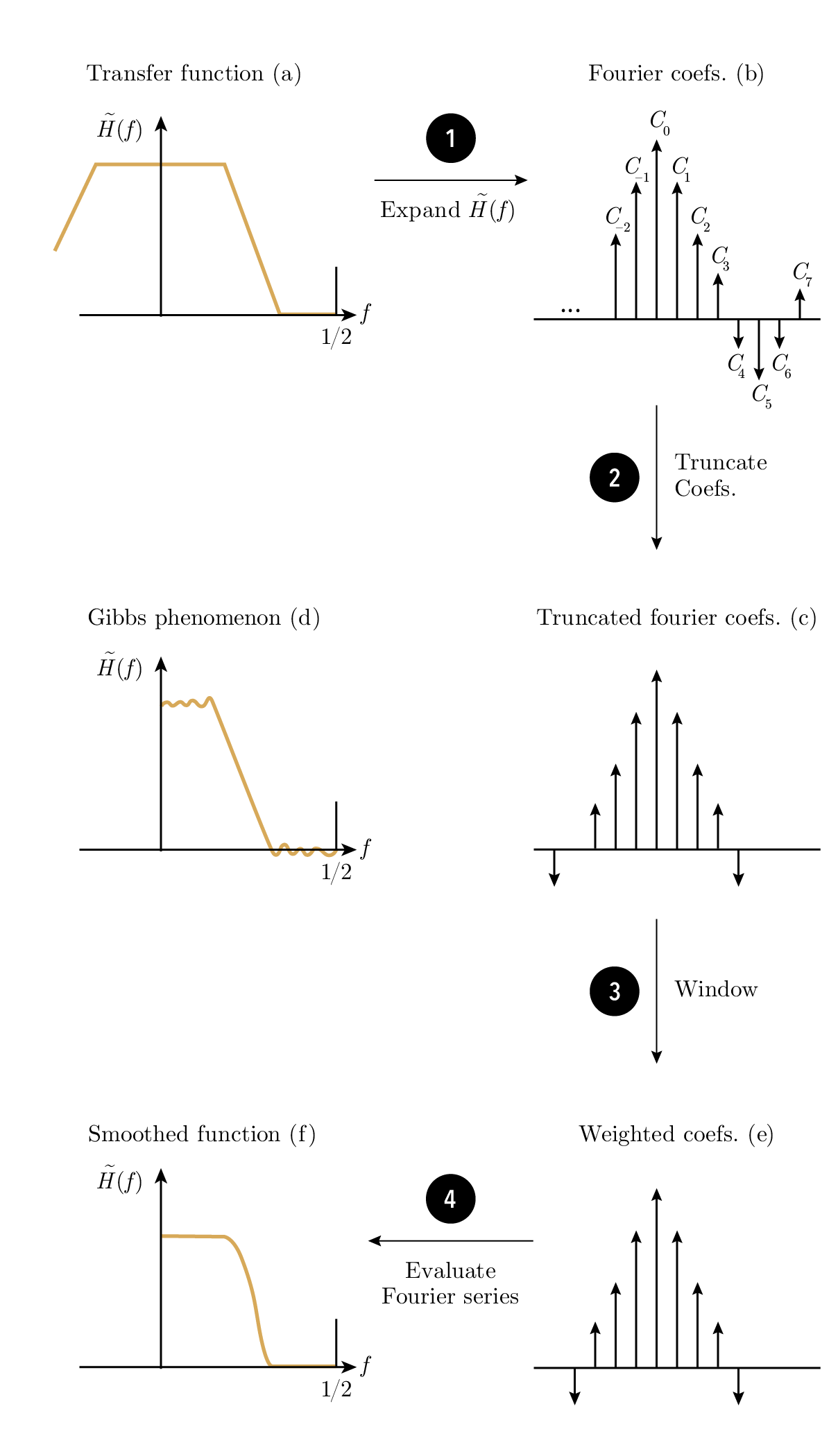
Figure 16.1—Truncating the infinite Fourier series (การตัดอนันต์อนุกรมฟูเรียร์)
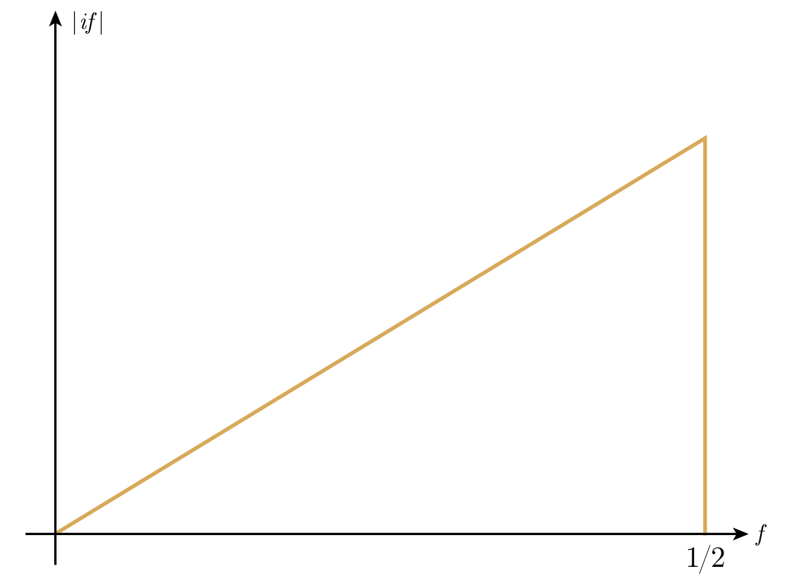
Figure 16.2—Amplification for differentiation (การขยายสัญญาณสำหรับการทำ differentiation)
สัมประสิทธิ์ของอนุกรมฟูเรียร์เชิงรูปแบบ ที่สอดคล้องกันนั้นคำนวณได้ง่าย เนื่องจาก integrand ของนิพจน์เหล่านั้นตรงไปตรงมา (ใช้ integration by parts เมื่อคุณมี derivative) สมมติว่าเราแทนอนุกรมในรูปของ complex exponentials แล้วสัมประสิทธิ์ของ filter ก็คือ Fourier coefficients ของ exponential terms ที่สอดคล้องกัน ที่มุมขวาบนของ Figure 16.1 เรามีภาพร่างของสัมประสิทธิ์เชิงสัญลักษณ์ (แน่นอนว่ามันเป็นจำนวนเชิงซ้อน)
ต่อไป เราต้องตัดอนันต์อนุกรมฟูเรียร์ให้เหลือ 2 N +1 พจน์ (หมายถึงใช้ rectangular window) ซึ่งแสดงใน Figure 16.1 พร้อมการแสดงแบบฟูเรียร์ทางซ้ายที่แสดง Gibbs effect
ประการที่สาม เราจะเลือก window เพื่อลบ Gibbs effect ที่แย่ที่สุดออกไป สัมประสิทธิ์ที่ผ่าน window แล้วจะแสดงที่มุมขวาล่าง พร้อมกับ digital filter สุดท้ายที่มุมซ้ายล่าง ในทางปฏิบัติ คุณควรปัดเศษสัมประสิทธิ์ของ filter ก่อนที่จะประเมิน transfer function เพื่อให้เห็นผลของมัน
ในวิธีการที่ร่างไว้ข้างต้น คุณต้องเลือกทั้ง N คือจำนวนพจน์ที่จะเก็บ และรูปทรงของ window ที่เฉพาะเจาะจง และถ้าสิ่งที่คุณได้ไม่เหมาะกับคุณ คุณก็ต้องเลือกใหม่ เป็นวิธีการออกแบบแบบ "ลองผิดลองถูก"
J.F. Kaiser ได้ให้วิธีการออกแบบที่หาได้ทั้ง N และสมาชิกของตระกูล windows ที่จะทำงานนั้นได้ คุณต้องระบุสองสิ่งนอกเหนือจากรูปทรง: ระยะทางแนวตั้งที่คุณยอมให้คลาดเคลื่อนจากอุดมคติได้ ซึ่งเรียกว่า δ และความกว้างของการเปลี่ยนผ่านระหว่าง pass band และ stop band ซึ่งเรียกว่า Δ F , Figure 16.3 .
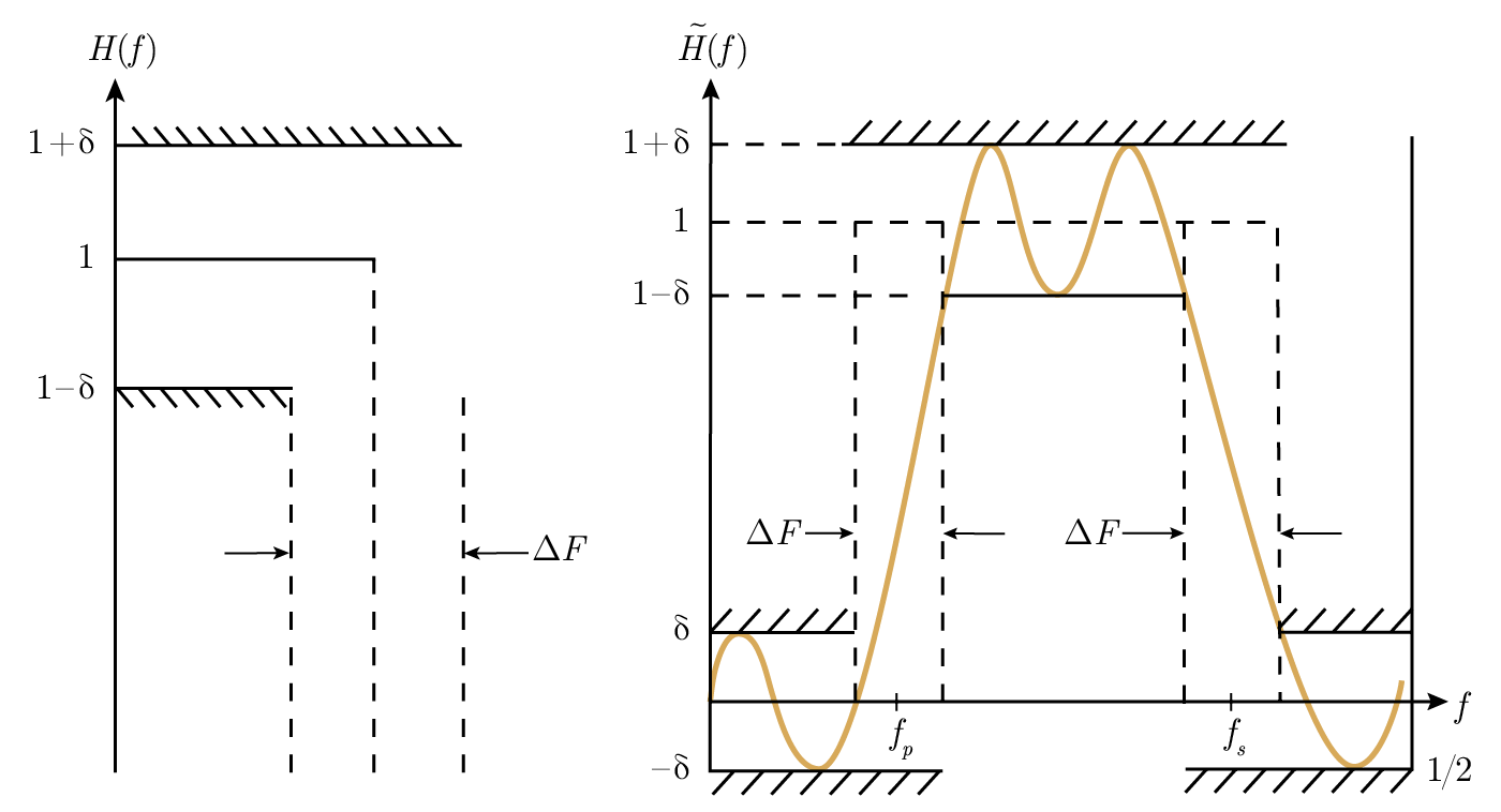
Figure 16.3—Band pass filter (ฟิลเตอร์แบนด์พาส)
สำหรับ band-pass filter โดยที่ f p คือความถี่ band-pass และ f s คือความถี่ band-stop ลำดับของสูตรการออกแบบคือ

ถ้า N ใหญ่เกินไป ให้หยุดและพิจารณาการออกแบบใหม่ มิฉะนั้นก็ดำเนินการคำนวณตามลำดับ

(ค่านี้ถูกพล็อตใน Figure 16.4 ) สัมประสิทธิ์ฟูเรียร์ดั้งเดิมสำหรับ band-pass filter กำหนดโดย


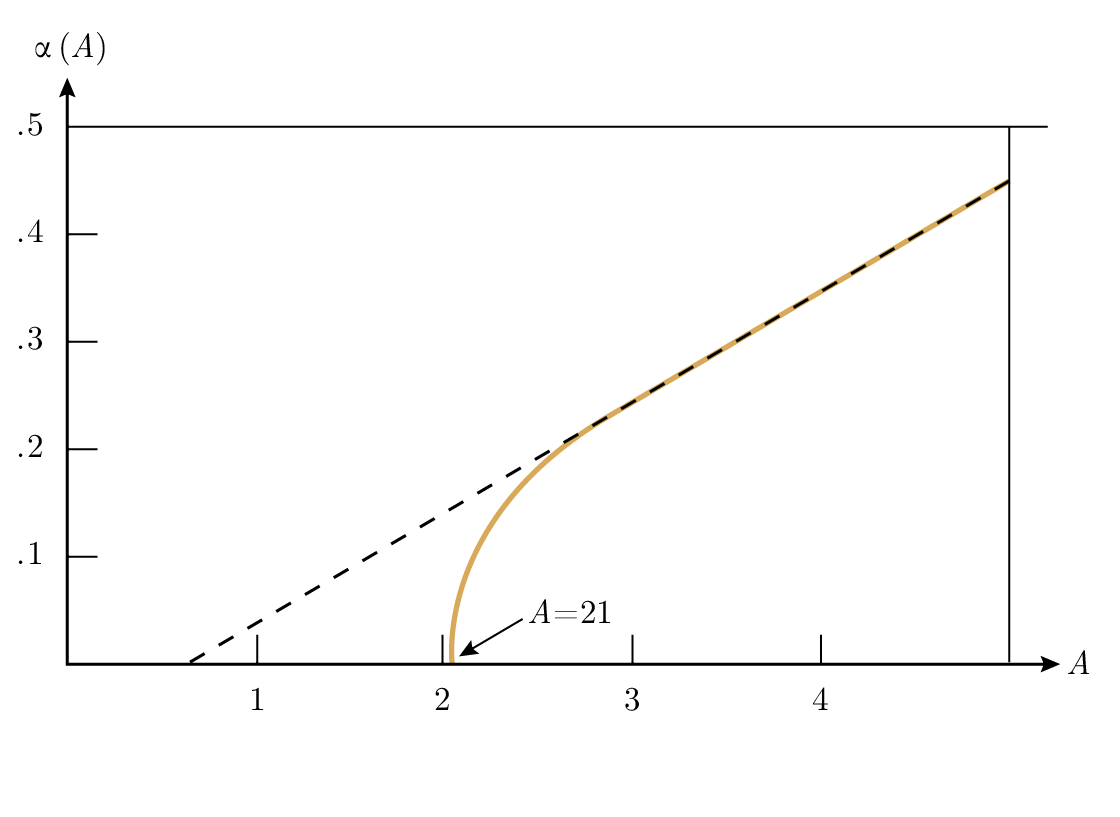
Figure 16.4— α ( A )
สัมประสิทธิ์เหล่านี้จะต้องคูณด้วยน้ำหนัก w k ที่สอดคล้องกันของ window

โดยที่

I 0 ( x ) คือ pure imaginary Bessel function อันดับ 0 สำหรับการคำนวณ คุณจะต้องใช้ไม่กี่พจน์ เนื่องจากมี (n ) !2 อยู่ในตัวส่วน ดังนั้นอนุกรมจึงลู่เข้าเร็ว
I 0 ( x ) คำนวณแบบ recursive ได้ดีที่สุด สำหรับ x ที่กำหนด พจน์ถัดไปของอนุกรมกำหนดโดย

สำหรับ low-pass หรือ high-pass ความถี่ใดความถี่หนึ่ง f p หรือ f s จะมีค่าขีดจำกัดที่เป็นไปได้ สำหรับ band-stop filter จะมีการเปลี่ยนแปลงเล็กน้อยในสูตรสำหรับสัมประสิทธิ์ c k .
ลองดูสัมประสิทธิ์ของ Kaiser window, ค่า w k กัน:

เมื่อเราดูตัวเลขเหล่านี้ เราจะเห็นว่าสำหรับ α > 0 มันมีรูปร่างคล้าย raised cosine

และมีลักษณะคล้ายกับ von Hann และ Hamming windows จะมี "platform" เมื่อ A > 21 สำหรับ A > 21 แล้ว a \= 0 , w k ทั้งหมดมีค่าเท่ากับ 1 และมันคือ Lanczos-type window เมื่อ A เพิ่มขึ้น platform ก็จะค่อยๆ ปรากฏขึ้น ดังนั้น Kaiser window จึงมีคุณสมบัติคล้ายกับ windows ยอดนิยมอื่นๆ หลายตัว และ window ที่คุณใช้จะถูกกำหนดจากข้อกำหนดของคุณผ่าน window ของเขา แทนที่จะเป็นการเดาหรืออคติ
Kaiser หาสูตรเหล่านี้ได้อย่างไร? ส่วนหนึ่งคือการลองผิดลองถูก เขาเริ่มต้นด้วยสมมติว่ามี discontinuity เดียว และรันเคสจำนวนมากบนคอมพิวเตอร์เพื่อดูทั้ง rise time Δ F และความสูงของ ripple δ ด้วยการคิดค่อนข้างมาก บวกกับความอัจฉริยะ และสังเกตว่าเมื่อเป็นฟังก์ชันของ A เมื่อ A เพิ่มขึ้น เราจะเปลี่ยนจาก Lanczos window ( A < 21) ไปเป็น platform ที่มีความสูงเพิ่มขึ้น 1/ I 0 (α) โดยหลักการแล้วเขาต้องการ prolate spheroidal function แต่เขาสังเกตว่ามันสามารถประมาณได้อย่างแม่นยำ สำหรับค่าของเขา โดยใช้ I 0 ( x ) เขาพล็อตผลลัพธ์และประมาณฟังก์ชันต่างๆ ผมถามเขาว่าเขาได้เลขชี้กำลัง 0.4 มาได้อย่างไร เขาตอบว่าเขาลอง 0.5 แล้วมันใหญ่เกินไป และ 0.4 ซึ่งเป็นตัวเลือกถัดไปตามธรรมชาติ ดูเหมือนจะพอดีมาก นี่เป็นตัวอย่างที่ดีของการใช้สิ่งที่รู้จักกันบวกกับคอมพิวเตอร์เป็นเครื่องมือทดลอง แม้แต่ในงานวิจัยเชิงทฤษฎี เพื่อให้ได้ผลลัพธ์ที่มีประโยชน์มาก
วิธีการของ Kaiser จะล้มเหลวเป็นครั้งคราว เพราะจะมีมากกว่าหนึ่ง edge (อันที่จริงแล้ว มีภาพสะท้อนสมมาตรของ edge ที่ส่วนลบของเส้นความถี่) และ ripples จาก edges ที่ต่างกันอาจรวมกันโดยบังเอิญและทำให้ filter ripples เกินค่าที่กำหนด ในกรณีนี้ ซึ่งเกิดขึ้นไม่บ่อย คุณก็แค่ทำการออกแบบซ้ำด้วย tolerance ที่เล็กลง โปรแกรมทั้งหมดสามารถทำงานได้อย่างง่ายดายบนเครื่องคอมพิวเตอร์แบบพกพาดั้งเดิมอย่าง ti – 59 ไม่ต้องพูดถึงบน pc สมัยใหม่
ต่อไปเราจะพูดถึง finite Fourier series . เป็นข้อเท็จจริงที่น่าทึ่งที่ฟังก์ชันฟูเรียร์ตั้งฉากกัน ไม่เพียงแต่บน segment ของเส้นตรงเท่านั้น แต่สำหรับชุดจุดที่เว้นระยะเท่ากันแบบ discrete ใดๆ ด้วย ดังนั้นทฤษฎีจะดำเนินไปในลักษณะเดียวกัน ยกเว้นว่าจะมีสัมประสิทธิ์ในอนุกรมฟูเรียร์ได้มากเท่ากับจำนวนจุดเท่านั้น ในกรณีของ 2 N จุด ซึ่งเป็นกรณีทั่วไป จะมีพจน์ความถี่สูงสุดเพียงพจน์เดียวเท่านั้น นั่นคือ cosine term (sine term จะเป็นศูนย์ที่จุดตัวอย่าง) สัมประสิทธิ์ถูกกำหนดจากผลรวมของจุดข้อมูลคูณด้วยฟังก์ชันฟูเรียร์ที่เหมาะสม การแสดงผลที่ได้จะสร้างข้อมูลดั้งเดิมขึ้นมาใหม่ได้ ภายในขอบเขตของ roundoff
ในการคำนวณ expansion จะต้องใช้ 2 N พจน์ แต่ละพจน์มีการคูณและบวก 2 N ครั้ง ดังนั้นจึงต้องใช้การดำเนินการคูณและบวกประมาณ (2 N ) 2 ครั้ง แต่ด้วยการ (1) ทำการบวกและลบพจน์ที่มีตัวคูณเดียวกันก่อนที่จะทำการคูณ และ (2) สร้างความถี่ที่สูงขึ้นโดยการคูณความถี่ที่ต่ำกว่า ทำให้ fast Fourier transform ( fft ) เกิดขึ้น โดยต้องการการดำเนินการประมาณ N log N ครั้ง การลดปริมาณการคำนวณนี้ได้เปลี่ยนแปลงวิทยาศาสตร์และวิศวกรรมศาสตร์ในหลายด้านไปอย่างมาก — สิ่งที่เคยเป็นไปไม่ได้ทั้งในด้านเวลาและต้นทุน ปัจจุบันกลายเป็นเรื่องที่ทำกันเป็นประจำ
ตอนนี้ขอเล่าเรื่องจากชีวิตจริงอีกเรื่องหนึ่ง คุณทุกคนคงเคยได้ยินเกี่ยวกับ fast Fourier transform และบทความของ Tukey-Cooley บางครั้งมันถูกเรียกว่า Tukey-Cooley transform หรือ algorithm Tukey ได้แนะนำแนวคิดพื้นฐานของ fft ให้ผมฟังแบบคร่าวๆ ตอนนั้นผมมี ibm Card Programmed Calculator ( cpc ) และการดำเนินการแบบ "butterfly" ทำให้มันเป็นไปไม่ได้เลยที่จะทำกับอุปกรณ์ที่ผมมี ไม่กี่ปีต่อมาผมมี ibm 650 ที่โปรแกรมได้ภายใน และเขาได้พูดถึงมันอีกครั้ง สิ่งที่ผมจำได้คือมันเป็นหนึ่งในไอเดียไม่กี่อย่างของ Tukey ที่แย่; ผมลืมไปโดยสิ้นเชิงว่าทำไมมันถึงแย่ — นั่นก็เพราะอุปกรณ์ที่ผมมีในตอนนั้น ดังนั้นผมจึงไม่ได้ทำ fft แม้ว่าหนังสือที่ผมตีพิมพ์ไปแล้ว (1961) แสดงให้เห็นว่าผมรู้ข้อเท็จจริงที่จำเป็นทั้งหมด และสามารถทำได้อย่างง่ายดาย!
บทเรียน: เมื่อคุณรู้ว่าบางสิ่งไม่สามารถทำได้ ก็ให้จดจำเหตุผลสำคัญว่าทำไมมันถึงทำไม่ได้ด้วย เพื่อที่ภายหลัง เมื่อสถานการณ์เปลี่ยนไป คุณจะได้ไม่พูดว่า "มันทำไม่ได้" นึกถึงความผิดพลาดของผมสิ! จะมีใครโง่ไปกว่านี้อีกไหม? โชคดีสำหรับอัตตาของผม มันเป็นความผิดพลาดที่พบบ่อย (และผมก็ทำมันมากกว่าหนึ่งครั้ง) แต่เนื่องจากความพลาดของผมเกี่ยวกับ fft ทำให้ผม sensitivity กับเรื่องนี้มากในตอนนี้ ผมยังสังเกตเห็นเมื่อคนอื่นทำมัน — ซึ่งบ่อยเกินไป! โปรดจำเรื่องราวว่าผมโง่แค่ไหนและสิ่งที่ผมพลาดไป และอย่าทำผิดพลาดนั้นด้วยตัวคุณเอง เมื่อคุณตัดสินใจว่าบางสิ่งเป็นไปไม่ได้ อย่าพูดในภายหลังว่ามันยังคงเป็นไปไม่ได้โดยไม่ทบทวน รายละเอียด ทั้งหมดว่าทำไมคุณถึงพูดถูกตั้งแต่แรกว่ามันทำไม่ได้
ตอนนี้ผมต้องพูดถึงหัวข้อที่ละเอียดอ่อนอย่าง power spectra ซึ่งคือผลรวมของกำลังสองของสัมประสิทธิ์ทั้งสองของความถี่ที่กำหนดในโดเมนจริง หรือกำลังสองของค่าสัมบูรณ์ในสัญกรณ์เชิงซ้อน การตรวจสอบจะทำให้คุณเชื่อว่าปริมาณนี้ไม่ได้ขึ้นอยู่กับจุดกำเนิดของเวลา แต่ขึ้นอยู่กับสัญญาณเท่านั้น ตรงกันข้ามกับการพึ่งพาของสัมประสิทธิ์ต่อตำแหน่งของจุดกำเนิด สเปกตรัมมีบทบาทสำคัญมากในประวัติศาสตร์ของวิทยาศาสตร์และวิศวกรรมศาสตร์ เส้นสเปกตรัมคือสิ่งที่เปิดกล่องดำของอะตอมและทำให้ Bohr มองเห็นข้างใน กลศาสตร์ควอนตัมใหม่ที่เริ่มต้นราวปี 1925 ได้ปรับเปลี่ยนสิ่งต่างๆ เล็กน้อย แต่สเปกตรัมยังคงเป็นกุญแจสำคัญ เรายังวิเคราะห์กล่องดำเป็นประจำโดยการตรวจสอบสเปกตรัมของ input และสเปกตรัมของ output พร้อมกับความสัมพันธ์ต่างๆ เพื่อทำความเข้าใจสิ่งที่อยู่ภายใน — ไม่ใช่ว่าจะมีภายในที่ตายตัวเสมอไป แต่โดยทั่วไปเราได้รับเบาะแสมากพอที่จะสร้างทฤษฎีใหม่
มาวิเคราะห์อย่างระมัดระวังว่าเราทำอะไรและความหมายของมัน เพราะว่า สิ่งที่เราทำมีอิทธิพลอย่างมากต่อสิ่งที่เรามองเห็น โดยปกติแล้ว ในจินตนาการของเราอย่างน้อยที่สุด ก็จะมีสัญญาณต่อเนื่อง ซึ่งมักจะไม่มีที่สิ้นสุด และเราเก็บตัวอย่างในเวลาที่มีความยาว 2 L นี่เหมือนกับการคูณสัญญาณด้วย Lanczos window หรือ box car ถ้าคุณชอบ นั่นหมายความว่าสัญญาณดั้งเดิมถูก convolved กับฟังก์ชันที่สอดคล้องกันในรูป (sin x )/ x , Figure 16.5 — ยิ่งสัญญาณยาวเท่าไหร่ ลูปลของ (sin x )/ x ก็ยิ่งแคบลงเท่านั้น เส้นสเปกตรัมบริสุทธิ์แต่ละเส้นถูก smear ออกเป็นรูปร่าง (sin x )/ x ของมัน
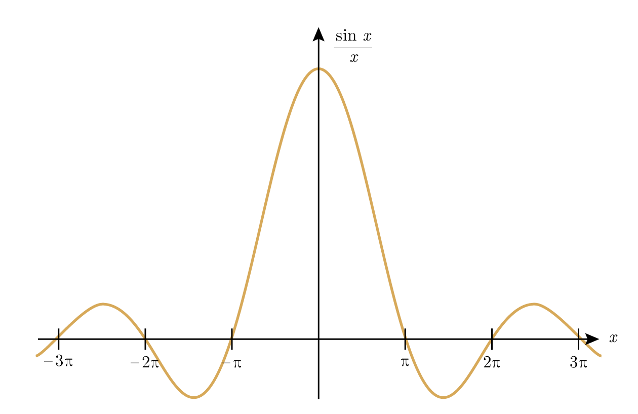
Figure 16.5—Graph of sin x / x (กราฟของ sin x / x)
ต่อไปเราจะสุ่มตัวอย่างที่ระยะห่างเท่ากันในเวลา และความถี่ที่สูงกว่าทั้งหมดจะถูก aliased ไปเป็นความถี่ที่ต่ำกว่า เห็นได้ชัดว่าการสลับลำดับการดำเนินการสองอย่างนี้ — สุ่มตัวอย่างแล้วจำกัดช่วง — จะให้ผลลัพธ์เดียวกัน และอย่างที่ผมเคยพูดไว้ ผมเคยคำนวณรายละเอียดพีชคณิตทั้งหมดอย่างละเอียดเพื่อให้แน่ใจกับตัวเองว่าสิ่งที่ผมคิดว่าต้องเป็นจริงตามทฤษฎีนั้นเป็นจริงในทางปฏิบัติ
จากนั้นเราใช้ fft ซึ่งเป็นแค่วิธีที่ชาญฉลาดและแม่นยำในการหาสัมประสิทธิ์ของ finite Fourier series แต่เมื่อเราสมมติการแทนแบบ finite Fourier series เรากำลังทำให้ฟังก์ชันเป็นคาบ — และคาบนั้นก็คือขนาดของช่วงสุ่มตัวอย่างคูณกับจำนวนตัวอย่างที่เราเก็บ! โดยทั่วไปคาบนี้ไม่มีอะไรเกี่ยวข้องกับคาบในสัญญาณดั้งเดิม เราบังคับให้ความถี่ที่ไม่ใช่ฮาร์มอนิกทั้งหมดกลายเป็นความถี่ฮาร์มอนิก — เราบังคับให้ continuous spectrum กลายเป็น line spectrum! การบังคับนี้ไม่ใช่ผลกระทบเฉพาะที่ แต่ดังที่คุณสามารถคำนวณได้ง่ายๆ ความถี่ที่ไม่ใช่ฮาร์มอนิกจะกระจายไปยังความถี่อื่นๆ ทั้งหมด โดยมากที่สุดไปยังความถี่ที่อยู่ติดกัน แต่ก็กระจายไปยังความถี่ที่ไกลออกไปอย่างมีนัยสำคัญ
ผมได้ละเลยเคล็ดลับทางสถิติมาตรฐานในการลบค่าเฉลี่ย ไม่ว่าจะเพื่อความสะดวกหรือด้วยเหตุผลเกี่ยวกับ calibration สิ่งนี้จะลดปริมาณของความถี่ 0 ในสเปกตรัมให้เป็น 0 และสร้าง discontinuity ที่มีนัยสำคัญในสเปกตรัม ถ้าคุณใช้ window ในภายหลัง คุณก็แค่ smear มันไปยังความถี่ใกล้เคียง ในการประมวลผลข้อมูลให้ Tukey ผม regularly ลบแนวโน้มเชิงเส้นและแม้แต่แนวโน้มพาราโบลาจากข้อมูลบางอย่างเกี่ยวกับการบินของเครื่องบินหรือขีปนาวุธ แล้ววิเคราะห์ส่วนที่เหลือ แต่สเปกตรัมของผลรวมของสัญญาณสองสัญญาณไม่ใช่ผลรวมของสเปกตรัม — ไม่ใช่แม้แต่ใกล้เคียง! เมื่อคุณบวกสองฟังก์ชัน ความถี่แต่ละความถี่จะถูกบวก เชิงพีชคณิต และมันอาจเสริมหรือหักล้างกัน และให้ผลลัพธ์ที่ผิดพลาดโดยสิ้นเชิง! ไม่มีใครที่ผมรู้จักมีคำตอบที่สมเหตุสมผลต่อข้อโต้แย้งของผมที่นี่ — เรายังคงทำมัน partly เพราะเราไม่รู้จะทำอะไรอื่น — แต่ trend line มี discontinuity ใหญ่ที่ปลาย (จำไว้ว่าเราสมมติว่าฟังก์ชันทั้งหมดเป็นคาบ) ดังนั้นสัมประสิทธิ์ของมันจึงลดลงแบบ 1/ k ซึ่งไม่เร็วเลย!
มาดูทฤษฎีกัน ทุกสเปกตรัมของ noise จริงจะลดลงอย่างรวดเร็วพอสมควรเมื่อคุณไปถึงความถี่อนันต์ มิฉะนั้นมันจะมีพลังงานไม่จำกัด Figure 16.6 แต่กระบวนการ sampling จะ alias ความถี่ที่สูงกว่าไปเป็นความถี่ที่ต่ำกว่า และการ folding ดังที่แสดงมีแนวโน้มที่จะสร้างสเปกตรัมแบบราบ — จำไว้ว่า ความถี่เมื่อถูก aliased จะถูกบวกเชิงพีชคณิต ดังนั้นเราจึงมีแนวโน้มที่จะเห็นสเปกตรัมแบบราบสำหรับ noise และถ้ามันราบ เราก็เรียกมันว่า white noise โดยปกติสัญญาณจะอยู่ในความถี่ต่ำเป็นหลัก นี่เป็นจริงด้วยเหตุผลหลายประการ รวมถึง "over-sampling" (การสุ่มตัวอย่างบ่อยกว่าที่กำหนดโดย Nyquist theorem) และหมายความว่าเราสามารถทำ averaging เพื่อลด instrumental errors ดังนั้นสเปกตรัมทั่วไปจะมีลักษณะดังที่แสดงใน Figure 16.6 ดังนั้นจึงมีความชุกของ low-pass filters เพื่อกำจัด noise ไม่มีวิธีเชิงเส้นใดที่สามารถแยกสัญญาณจาก noise ที่ความถี่เดียวกันได้ แต่ความถี่ที่เกินกว่าสัญญาณสามารถถูกกำจัดได้ด้วย low-pass filter ดังนั้น เมื่อเรา "over-sample" เรามีโอกาสที่จะกำจัด noise ได้มากขึ้นด้วย low-pass filter
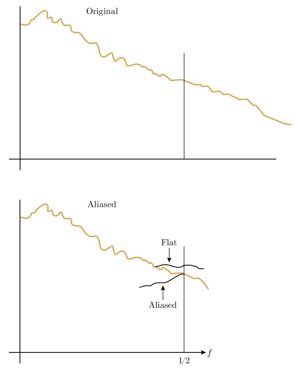
Figure 16.6—Typical spectrum (สเปกตรัมทั่วไป)
จำไว้ว่า มีความเข้าใจโดยนัยว่าเรากำลังประมวลผลระบบเชิงเส้น การวิเคราะห์ฟูเรียร์ตลาดหุ้นแบบเก่า ที่เปิดเผยว่ามีเพียง white noise ถูกตีความว่าหมายถึงไม่มีทางทำนายราคาหุ้นในอนาคตได้ — และนี่ถูกต้องก็ต่อเมื่อคุณตั้งใจจะใช้ตัวทำนายเชิงเส้นแบบง่ายเท่านั้น แต่มันไม่ได้พูดอะไรเกี่ยวกับการใช้ nonlinear predictors ในทางปฏิบัติ นี่เป็นการตีความผลลัพธ์ที่ผิดอย่างแพร่หลายอีกครั้ง เนื่องจากขาดความเข้าใจพื้นฐานเบื้องหลังเครื่องมือทางคณิตศาสตร์ และรู้เพียงแค่เครื่องมือเท่านั้น ความรู้เพียงเล็กน้อยเป็นสิ่งอันตราย — โดยเฉพาะถ้าคุณขาด พื้นฐาน!
ผมพูดอย่างระมัดระวังในการบรรยายเปิดเกี่ยวกับ digital filters ว่าผม คิด ว่าตอนนั้นผมไม่รู้อะไรเกี่ยวกับมันเลย สิ่งที่ผมไม่รู้คือการที่ตอนนั้นผมไม่รู้เกี่ยวกับการออกแบบ recursive digital filter ทำให้ผมสร้างมันขึ้นมาได้อย่างมีประสิทธิภาพเมื่อผมตรวจสอบทฤษฎีของวิธีการ predictor-corrector ในการแก้สมการเชิงอนุพันธ์สามัญเชิงตัวเลข ตัว corrector นั้นแทบจะเป็น recursive digital filter!
ในขณะที่ศึกษาวิธีการ integrate ระบบสมการเชิงอนุพันธ์สามัญเชิงตัวเลข ผมไม่ถูกจำกัดด้วยความคิด preconceived เกี่ยวกับ digital filters และในไม่ช้าผมก็ตระหนักว่า bounded input ในภาษาของผู้เชี่ยวชาญด้าน filter สามารถสร้าง unbounded output ได้ ถ้าคุณกำลัง integrate — ซึ่งพวกเขาบอกว่ามัน unstable แต่ชัดเจนว่ามันคือสิ่งที่คุณต้องมีถ้าคุณต้องการ integrate; แม้แต่ค่าคงที่ก็จะสร้างการเติบโตเชิงเส้นใน output อันที่จริง เมื่อต่อมาผมต้องเผชิญกับการ integrate trajectory ลงไปยังพื้นผิวดวงจันทร์ ที่ซึ่งไม่มีอากาศ จึงไม่มี drag จึงไม่มี first derivatives อย่างชัดเจนในสมการ และต้องการใช้ประโยชน์จากสิ่งนี้โดยใช้สูตรที่เหมาะสมสำหรับ numerical integration ผมพบว่าผมต้องมีการเติบโตของ error แบบ quadratic; ข้อผิดพลาดจากการปัดเศษเล็กน้อยในการคำนวณ acceleration จะไม่ถูกแก้ไขและจะนำไปสู่ error แบบ quadratic ในตำแหน่ง — error ใน acceleration ทำให้เกิดการเติบโตแบบ quadratic ในตำแหน่ง นั่นคือธรรมชาติของปัญหา แตกต่างจากบนโลกที่ air drag ให้ feedback correction บางอย่างกับค่าความเร่งที่ผิด และจึงให้การแก้ไข error ในตำแหน่งบางส่วน
ดังนั้นจนถึงทุกวันนี้ผมยังมีทัศนคติว่า stability ใน digital filters หมายถึง "ไม่ใช่ exponential growth" จาก bounded inputs แต่อนุญาตให้ polynomial growth และนี่ไม่ใช่เกณฑ์ stability มาตรฐานที่ได้จาก classical analog filters ซึ่งถ้ามันไม่ bounded คุณจะละลายอุปกรณ์ — และอย่างไรก็ตาม พวกเขาไม่เคยคิดอย่างจริงจังเกี่ยวกับ integration ในฐานะกระบวนการของ filter
เราจะพูดถึงหัวข้อสำคัญของ recursive filters ซึ่งจำเป็นสำหรับ integration ในบทต่อไป